SAP Datasphere: why expose data to SAC through an Analytic Model
Fact view, Analytical Dataset or Analytic Model in SAP Datasphere: the differences and how to organize your layers for consumption in SAP Analytics Cloud.
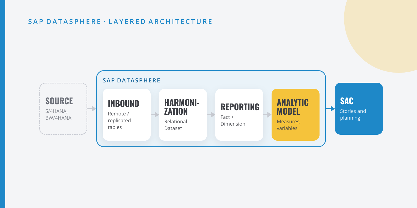
Table of contents
When you start with SAP Datasphere coming from BW, the temptation is to build a view, mark it as exposed for consumption and connect SAP Analytics Cloud directly. It works… until you need restricted key figures, variables or currency conversion. That is where the Analytic Model comes in.
Semantic usage changes everything
In the Data Builder, every graphical or SQL view has a semantic usage. The ones you will use most:
- Relational Dataset: a “normal” table or view, with no analytical semantics.
- Dimension: master data with attributes, texts and associated hierarchies.
- Text and Hierarchy: language-dependent texts and parent-child hierarchies.
- Fact: the transactional dataset with measures and associations to dimensions.
- Analytical Dataset: the older type for exposing data directly to SAC.
What the Analytic Model brings
The Analytic Model is built on top of a Fact view and is, in practice, the closest thing to a BW query:
- Calculated and restricted measures, just like calculated/restricted key figures in BEx.
- Count distinct and exception aggregation.
- Variables: filter variables, variables for restricted measures or reference-date variables.
- Declarative currency and unit conversion.
- Choosing which dimensions and attributes are exposed, without touching the views underneath.
- Built-in data preview to validate before anything reaches SAC.
A layered architecture that works
The setup that is working best for me on projects:
- Inbound: remote or replicated tables from S/4HANA or BW/4HANA, with no logic.
- Harmonization: Relational Dataset views that clean, unify and apply business rules.
- Reporting: Fact and Dimension views with well-defined associations.
- Consumption: one or more Analytic Models per use case, which are the only thing SAC sees.
That way, changing a consumption model does not break anything underneath, and each layer has a single responsibility.
Example: a Fact view in SQL
A simple SQL view that we would then mark as Fact and associate with the hotel and date dimensions:
SELECT "HOTEL_ID", "STAY_DATE", "MARKET_SEGMENT", "CURRENCY", SUM("ROOM_NIGHTS") AS "ROOM_NIGHTS", SUM("ROOM_REVENUE") AS "ROOM_REVENUE"FROM "V_HARM_RESERVATIONS"WHERE "STATUS" <> 'CANCELLED'GROUP BY "HOTEL_ID", "STAY_DATE", "MARKET_SEGMENT", "CURRENCY"In the Analytic Model we would then add ADR as a calculated measure (ROOM_REVENUE / ROOM_NIGHTS) with the right aggregation, plus a variable for the stay date range.
Checklist before publishing to SAC
- The Fact view has measures with their aggregation type and associations to every dimension.
- Dimensions have texts and, where relevant, hierarchies.
- The Analytic Model exposes only the attributes users need.
- Restricted measures and variables have been tested with the data preview.
- Permissions (Data Access Controls) are applied in the reporting views, not in SAC.
With this in place, SAC becomes a visualization and planning layer, and the logic lives where it belongs: in Datasphere.